Why is a teacher like a video game developer?

No, this isn’t a raven and writing desk riddle. Teachers and game developers have more in common than you might think!

You need to assume that any instructions you give will be promptly ignored

The classroom is like a giant sandbox game. You need to think of every conceivable action that might be taken by the player/student and ensure there are some appropriate consequences in place. Preferably realistic ones too. You could go with the insta-death lava to restrict movement if you want, but expect some angry phone calls from parents.

For every hour you spend planning you wish you had three

Seriously. The difference between a well planned project/lesson is night and day. Unfortunately, I don’t think my principal will go for the 1:1 class period to prep period schedule…

For every hour you spend working, you spend another hour documenting what you did

It’s called CYA: Cover. Your. WE DON’T SAY THAT AT SCHOOL!

Would it be out of line for me to start tracking student behaviors in Bugzilla?

You refer to 60+ hour work weeks as “normal”

Veterans of the video game industry are no strangers to “crunch time”. It’s the unavoidable time period before the end of a project where “get it out the door” fever starts to set in. The title ships, you briefly reflect on what worked and what didn’t, then the next project starts and before you know it you’re back in “crunch” mode. Teachers refer to this cycle as “a school day”.

There’s a ton of little things you’d like to fix, you just don’t have the time

These are things that were probably noticed by some highly caffeinated tester in a poorly lit basement somewhere, added to the bug database, and ultimately stamped with those three fateful letters: WNF. Will. Not. Fix. “Yes, there’s a typo in question 4. GET OVER IT.”

RFC: Are geometric constructions still relevant?

Dear friends, fellow math teachers, game developers and artists.

I’ve got this little dilemma I’m wondering if you could help me with. You see, part of my geometry curriculum deals with compass and straightedge constructions. My colleagues have suggested that this is a topic we, not exactly skip, but… I dunno what the appropriate word here is… trim? They argue that it’s largely irrelevant for our students, is overly difficult, and represents a minimal component of the SOL test. And I don’t think they’re wrong. I haven’t used a compass and straightedge since I left high school either.

However, something about these constructions strikes as beautiful. Part of me thinks that’s enough reason to include them, but it also got me thinking about more practical applications of them. Where did I use them? I used them making video games. Video games build worlds out of “lines” and “spheres”. Beautiful worlds.

My question is this, do my 3D artist friends feel the same way? Do you remember your compass and straightedge constructions? Do you use them, or some derivation thereof, in your everyday work? Are you glad to have learned them? Or are the elementary constructions made so trivial in modern 3D modeling software that you don’t even think about them?

Please comment and share.

And now for taste of things to come…

It’s been a while since my last post, but I’m still here! A lot has happened in the past 6 months and I’m not trying to be neglectful of my blogging. In an effort to give myself some added motivation, I’m going to try to outline some of the things I have planned for this blog. By making this list public, hopefully I’ll feel pressured to hold myself to it. So, without further ado, here’s what you have to look forward to in the months to come:

I’m currently working on a custom WordPress theme for this blog. It’s taking a bit longer than anticipated, but it’s coming!
I’ve spent a good deal of time transitioning my courses to use OER materials. I wanted to take some time to reflect on the transition from MyMathLab to MyOpenMath and what the future may hold.
I’ve experimented in the past with automating my course syllabus creation. Now, I’m trying to take this one step further and generate an entire course. I don’t know how far I’m going to get with this, but would like to at least do an article about how I think LMSs could save instructors a great deal of time through dynamic course data.
It’s been a year since my foray into local politics. I’d like to take a look back on what happened since then.
Lately, I’ve been playing a bit of FPS as opposed to my usual RPGs. It’s given me ideas for some new metagaming posts.
Finally, and perhaps the biggest news, I’ve been offered a new job! I don’t want to give away too much yet, but let’s just say there’s potentially going to be a lot more math lessons here in the future! I do, however, feel obliged to reiterate that this is my personal blog and the views expressed here do not reflect the positions of any of my employers: past, present or future.

Anyways, I hope there’s some exciting things to come. Thanks for reading!

The Future of AI: 13 year old Ukrainian boy Looking for Guild?

I recently finished reading Michio Kaku’s The Future of the Mind and found it very thought provoking. A combination of cutting-edge advances in psychology, artificial intelligence and physics, mixed together with numerous pop-culture references made for a very informative and inspiring read. Many of the ideas presented seemed very reminiscent of the narratives in The Mind’s I, but with a greater emphasis on the practicality of technological advances. While I would no doubt recommend it to an interested reader, I don’t exactly intend for this post to turn into a book review. This is more of a personal reflection on some of my thoughts while reading it.

Defining Consciousness: Kaku vs Jaynes

My first point of intrigue begins with Kaku’s definition of consciousness, which he calls the “space-time theory of consciousness”:

Consciousness is the process of creating a model of the world using multiple feedback loops in various parameters (e.g., in temperature, space time, and relation to others), in order to accomplish a goal (e.g. find mates, food, shelter).

Consciousness is a notoriously difficult phenomenon to define, as this is as good of a definition as any in the context of the discussion. What’s interesting about this definition is that it begins with a very broad base and scales upward. Under Kaku’s definition, even a thermostat has consciousness — although to the lowest possible degree. In fact, he defines several levels of consciousness and units of measurement within those levels. Our thermostat is at the lowest end of the scale, Level 0, as it has only a single feedback loop (temperature). Level 0 also includes other systems with limited mobility but more feedback variables such as plants. Level 1 consciousness adds spacial awareness reasoning, while Level 2 adds social behaviour. Level 3 finally includes human consciousness:

Human consciousness is a specific form of consciousness that creates a model of the world and then simulates it in time, by evaluating the past to simulate the future. This requires mediating and evaluating man feedback loops in order to make a decision to achieve a goal.

This definition is much closer to conventional usage of the word “consciousness”. However, for me this definition seemed exceptionally similar to a very specific definition I’d seen before. This contains all the essential components of Julian Jaynes’ definition in The Origin of Consciousness!

Jaynes argued that the four defining characteristics of consciousness are an analog “I”, (2) a metaphor “me”, (3) inner narrative, and (4) introspective mind-space. The “analog ‘I'” is similar to what Kaku describes as the brain’s “CEO” — the centralized sense of self that makes decisions about possible courses of action. Jaynes’ “introspective mind-space” is analogous to the “model of the world” in Kaku’s definition — our comprehensive understanding of the environment around us. The “metaphor ‘me'” is the representation of oneself within that world model that provides the “feedback loop” about the costs and benefits of hypothetical actions. Finally, what Jaynes’ describes as “inner narrative” serves as the simulation in Kaku’s model.

This final point is the primary difference between the two models. One of the possible shortcomings of Jaynes’ definition is that the notion of an “inner narrative” is too dependent on language. However, Kaku avoids this confusion by using the term “simulation”. Jaynes’ hypothesis was that language provided humanity with the mental constructs needed to simulate the future in a mental model. I think the differences in language are understandable given the respective contexts. Jaynes was attempting to establish a theory of how consciousness developed, while Kaku was attempting to summarize the model of consciousness that has emerged through brain imaging technology.

While I must admit some disappointment that Jaynes was not mentioned by name, it’s partly understandable. Jaynes’ theory is still highly controversial and not yet widely accepted in the scientific community. With Kaku’s emphasis on scientific advances, it might have been inappropriate for this book. Nevertheless, I’d be interested to hear Kaku’s thoughts on Jaynes’ theory after having written this book. Jaynes didn’t have the luxuries of modern neuroscience at his disposal, but that only makes the predictions of the theory more fascinating.

Artificial Intelligence (or the illusion thereof)

While I continued to read on, I happened to come across a news story proclaiming that Turing Test had been passed. Now, there’s a couple caveats to this claim. For one, this is not the first time a computer has successfully duped people into thinking it was human. Programs like ELIZA and ALICE have paved the way for more sophisticated chatterbots over the years. What makes this new bot, Eugene, so interesting is the way in which it confused the judges.

There’s plenty of room for debate about the technical merits of Eugene’s programming. However, I do think Eugene’s success is a marvel of social engineering. By introducing itself as a “13-year old Ukrainian boy”, the bot effectively lowers the standard for acceptable conversation. The bot is (1) pretending to be a child and (2) pretending to be a non-native speaker. Childhood naivety excuses a lack of knowledge about the world, while the secondary language excuses a lack of grammar. Together, these two conditions provide a cover for the most common shortcomings of chatterbots.

With Kaku’s new definition of consciousness in mind, I started to think more about the Turing Test and what it was really measuring. Here we have a “Level 0” consciousness pretending to be a “Level 3” consciousness by exploiting the social behaviors typical of a “Level 2” consciousness. I think it would be a far stretch to label Eugene as a “Level 3” consciousness, but does his social manipulation ability sufficiently demonstrate “Level 2” consciousness? I’m not really sure.

Before we can even answer that, Kaku’s model of consciousness poses an even more fundamental question. Is it possible to obtain “Level (n)” consciousness without obtaining “Level (n-1)”?

If yes, then maybe these levels aren’t really levels at all. Maybe one’s “consciousness” isn’t a scalar value, but a vector rating of each type of consciousness. A a human would score reasonably high in all four categories. Eugene is scoring high on Level 0, moderate on Level 2, and poor on Levels 1 and 3.

If no, then maybe the flaw in the A.I. development is that we’re attempting to develop social skills before spacial skills. This is partly due to the structure of the Turing Test. Perhaps, like the Jaynesian definition of consciousness, we’re focused a bit too much on the language. Maybe it’s time to replace the Turing Test with something a little more robust that takes multiple levels of consciousness into consideration.

The MMORPG-Turing Test

Lately I’ve been playing a bit of Wildstar. Like many popular MMORPGs, one of the significant problems facing the newly launched title is rampant botting. As games of this genre have grown in popularity, the virtual in-game currency becomes a commodity with real-world value. The time-consuming process behind the collection of in-game currency, or gold farming, provides ample motivation for sellers to automate the process using a computer program. Developers like Carbine are in a constant arms race to keep these bots out of the game to preserve the game experience for human players.

Most of these bots are incredibly simple. Many of them simply play back a pre-recorded set of keystrokes to the application. More sophisticated bots might read, and potentially alter, the game programs memory to perform more complicated actions. Often times these bots double as an advertising platform for the gold seller, and spam the in-game communication channels with the sellers website. It’s also quite common for the websites to contain key-loggers, as hijacking an existing player’s account is far more profitable than botting itself.

While I’m annoyed by bots as much as the next player, I must admit some level of intrigue with the phenomena. The MMORPG environment is essentially a Turing Test at an epic scale. Not only is the player-base of the game is on the constant look out for bot-like behavior, but also the developers implement algorithms for detecting bots. A successful AI would not only need to deceive humans, but also deceive other programs. It makes me wonder how sophisticated a program would need to be so that the bot would be indistinguishable from a human player. The odds are probably stacked against such a program.

Having played games of this type for quite some time, I’ve played with gamers who are non-native speaker or children and I’ve also seen my share of bots. While the “13 year old Ukrainian boy” ploy might work in a text-based chat, I think it would be much more difficult to pull off in an online game. It’s difficult to articulate, but human players just move differently. They react to changes in the environment in a way that is fluid and dynamic. On the surface, they display a certain degree of unpredictability while also revealing high-level patterns. Human players also show goal oriented behavior, but the goal of the player may not necessarily align with the goal of the game. It’s these type of qualities that I would expect to see from a “Level 1” consciousness.

Furthermore, online games have a complex social structure. Players have friends, guilds, and random acquaintances. Humans tend to interact differently depending on the nature of this relation. In contrast, a typical chatterbot treats everyone it interacts with the same. While some groups of players have very lax standards for who they play with, other groups hold very high standards for player ability and/or sociability. Eugene would have a very difficult time getting into an end-game raiding guild. If a bot could successfully infiltrate such a group, without their knowledge, it might qualify as a “Level 2” consciousness.

When we get to “Level 3” consciousness, that’s where things get tricky. The bot would not only need to understand the game world well enough to simulate the future, but it would also need to be able to communicate those predictions to the social group. It is, after all, a cooperative game and that communication is necessary to predict the behavior of other players. The bot also needs to be careful not to predict the future too well. It’s entirely possible for a bot to exhibit super-human behavior and consequently give itself away.

With those conditions for the various levels of consciousness, MMORPGs also enforce a form of natural selection on bots. Behave too predictably? Banned by bot detection algorithms. Fail to fool human players? Blacklisted by the community. Wildstar also potentially offers an additional survival resource in the form of C.R.E.D.D., which could require the bot to make sufficient in-game funds to continue its subscription (and consequently, its survival).

Now, I’m not encouraging programmers to start making Wildstar bots. It’s against the Terms of Service and I really don’t want to have to deal with anymore than are already there. However, I do think that an MMORPG-like environment offers a far more robust test of artificial intelligence than a simple text-based chat if we’re looking at consciousness using Kaku’s definition. Perhaps in the future, a game where players and bots can play side-by-side will exist for this purpose.

Conclusion

When I first started reading Kaku’s Future of the Mind, I felt like his definition of consciousness was merely a summary of the existing literature. As I continued reading, the depth of his definition seemed to continually grow on me. In the end, I think that it might actually offer some testable hypotheses for furthering AI development. I still think Kaku needs to read Jaynes’ work if he hasn’t already, but I also think he’s demonstrated that there’s room for improvement in that definition. Kaku certainly managed to stimulate my curiosity, and I call that a successful book.

Meta-Pokemon

In a previous post, I mentioned my fascination with Twitch Plays Pokemon (TPP). The reason behind this stems from the many layers of metagaming that take place in TPP. As I discussed in my previous post, the most basic definition of metagaming is “using resources outside the game to improve the outcome within the game”. However, there’s another definition of metagaming that has grown in usage thanks to Hofsteadter: “a game about a game”. This reflexive definition of metagaming is where the complexity of TPP begins to shine. Let’s take a stroll through some various types of metagaming taking place in TPP.

Outside resources

At the base level, we have players making use of a variety of outside resources to improve their performance inside the game. For Pokemon, the most useful resources might include maps, beastiaries, and Pokemon-type matchups. In TPP, many players also bring with them their own previous experiences with the game.

Game about a game

Pokemon itself is a metagame. Within the world of the game, the Pokemon League is its own game within the game. A Pokemon player is playing the role of a character who is taking part in game tournament. What makes TPP so interesting is that that it adds a game outside the game. Players in TPP can cooperate or compete for control of the game character. In effect, TPP is a meta-metagame: a game about a game about a game. Players in TPP are controlling the actions of a game character participating in a game tournament. It’s Pokemon-ception!

Gaming the population

Another use of metagaming is to take knowledge of the trends in player behaviors and utilize that information to improve the outcome within the game. In TPP, players would use social media sites such as Reddit to encourage the spread of certain strategies. Knowledge of social patterns in the general population TPP players enables a few players to guide the strategy of the collective in a desirable directions. Memes like “up over down” bring structure to an otherwise chaotic system and quickly become the dominant strategy.

Gaming the rules

One of my favorite pastimes in theory-crafting, which is itself a form of metagaming. Here, we take the rules of the game and look at possible strategies like a game. The method TPP used in the final boss fight is a perfect example of this. The boss is programmed to select a move type that the player’s pokemon is weak against and one of these moves deals no damage. By using a pokemon that is weak against this particular move, the boss is locked into a strategy that will never do any damage! Not only do the TPP players turn the rules of the game against it, but they also needed to organize the population to pull it off!

Gaming the population

Rule modification games

One of the defining characteristics of a game are the rules. The rules of Pokemon are well defined by the game’s code, but the rules of TPP are malleable. We can choose between “chaos” and “democracy”. Under chaos, every player input gets sent to the game. Under democracy, players vote on the next action to send. When we look at the selection of rules in terms of a game where we try to maximize viewers/participates, we get another type of metagaming.

Understanding Voter Regret

Lately I’ve been doing a little bit of research on voting methods. In particular, I’ve been fascinated by this idea of measuring Bayesian Regret. Unfortunately, many of the supporting links on rangevoting.org are dead. With a little detective work I managed to track down the original study and the supporting source code.

Looking at this information critically, one my concerns was the potential for bias in the study. This is the only study I could find taking this approach, and the information is hosted on a site that is dedicated to the support of the method proved most effective by the study. This doesn’t necessarily mean the result is flawed, but it’s one of the “red flags” I look for with research. With that in mind, I did what any skeptic should: I attempted it replicate the results.

Rather than simply use the provided source code, I started writing my own simulation from scratch. I still have some bugs to work out before I release my code, but the experience has been very educational so far. I think I’ve learned more about these voting methods by fixing bugs in my code than reading the original study. My initial results seem consistent with Warren Smith’s study but there’s still some kinks I need to work out.

What I’d like to do in this post is go over a sample election that came up while I was debugging my program. I’m hoping to accomplish a couple things by doing so. First, I’d like to explain in plain English what exactly the simulation is doing. The original study seems to be written with mathematicians in mind and I’d like for these results to be accessible to a wider audience. Second, I’d like to outline some of the problems I ran into while implementing the simulation. It can benefit me to reflect on what I’ve done so far and perhaps some reader out there will be able to provide input on these problems that will point me in the right direction.

Pizza Night at the Election House

It’s Friday night in the Election household, and that means pizza night! This family of 5 takes a democratic approach to their pizza selection and conducts a vote on what time of pizza they should order. They all agree that they should get to vote on the pizza. The only problem is that they can’t quite agree on how to vote. For the next 3 weeks, they’ve decided to try out 3 different election systems: Plurality, Instant-Runoff, and Score Voting.

Week 1: Plurality Voting

The first week they use Plurality Voting. Everyone writes down their favorite pizza and which ever pizza gets the most votes wins.

The youngest child votes for cheese. The middle child votes for veggie. The oldest votes for pepperoni. Mom votes for veggie, while dad votes for hawaiian.

With two votes, veggie pizza is declared the winner.

Mom and the middle child are quite happy with this result. Dad and the two others aren’t too excited about it. Because the 3 of them were split on their favorites, the vote went to an option that none of them really liked. They feel hopeful that things will improve next week.

Week 2: Instant Run-off Voting

The second week they use Instant Run-off Voting. Since the last election narrowed down the pizzas to four options, every lists those four pizzas in order of preference.

The youngest doesn’t really like veggie pizza, but absolutely hates pineapple. Ranks cheese 1st, pepperoni 2nd, veggie 3rd,and hawaiian last.

The middle child is a vegetarian. Both the hawaiian and pepperoni are bad options, but at least the hawaiian has pineapple and onions left over after picking off the ham. Ranks veggie 1st, cheese 2nd, hawaiian 3rd and pepperoni last.

The oldest child moderately likes all of them, but prefers fewer veggies on the pizza. Ranks pepperoni 1st, cheese 2nd, hawaiian 3rd and veggie last.

Dad too moderately likes all of them, but prefers the options with meat and slightly prefers cheese to veggie. Ranks hawaiian 1st, pepperoni 2nd, cheese 3rd and veggie last.

Mom doesn’t like meat on the pizza as much as Dad, but doesn’t avoid it entirely like the middle child. Ranks veggie 1st, cheese 2nd, pepperoni 3rd and hawaiian last.

Adding up the first place votes gives the same result as the first election: 2 for veggie, 1 for hawaiian, 1 for pepperoni and 1 for cheese. However, under IRV the votes for the last place pizza get transferred to the next ranked pizza on the ballot.

However, there’s something of a problem here. There’s a 3-way tie for last place!

A fight nearly breaks out in the Election house. Neither dad, the older or youngest want their favorite to be eliminated. The outcome of the election hinges on whose votes get transferred where!

Eventually mom steps in and tries to calm things down. Since the oldest prefers cheese to hawaiian and the youngest prefers pepperoni to hawaiian, it makes sense that dad’s vote for hawaiian should be the one eliminated. Since the kids agree with mom’s assessment, dad decides to go along and have his vote transferred to pepperoni.

Now the score is 2 votes for veggie, 2 votes for pepperoni, and 1 vote for cheese. Since cheese is now the lowest, the youngest childs vote gets transferred to the next choice: pepperoni. With a vote of 3 votes to 2, pepperoni has a majority and is declared the winner.

The middle child is kind of upset by this result because it means she’ll need to pick all the meat off her pizza before eating. Mom’s not exactly happy with it either, but is more concerned about all the fighting. They both hope that next week’s election will go better.

Week 3: Score Voting

The third week the Election family goes with Score Voting. Each family member assigns a score from 0 to 99 for each pizza. The pizza with the highest score is declared the winner. Everyone wants to give his/her favorite the highest score and least favorite the lowest, while putting the other options somewhere in between. Here’s how they each vote:

The youngest rates cheese 99, hawaiian 0, veggie 33 and pepperoni 96.

The middle child rates cheese 89, hawaiian 12, veggie 99 and pepperoni 0.

The oldest child rates cheese 65, hawaiian 36, veggie 0 and pepperoni 99.

Dad rates cheese 13, hawaiian 99, veggie 0 and pepperoni 55.

Mom rates cheese 80, hawaiian 0, veggie 99 and pepperoni 40.

Adding all these scores up, the finally tally is 346 for cheese, 147 for hawaiian, 231 for veggie and 290 for pepperoni. Cheese is declared the winner. Some of them are more happier than others, but everyone’s pretty much okay with cheese pizza.

Comparing the Results

Three different election methods. Three different winners. How do we tell which election method is best?

This is where “Bayesian Regret” comes in.

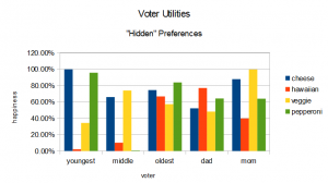
With each of these 3 elections, we get more and more information about the voters. First week, we get their favorites. Second week, we get an order of preference. Third week, we get a magnitude of preference. What if we could bypass the voting altogether and peak instead the voter’s head to see their true preferences? For the family above, those preferences would look like this:

	cheese	hawaiian	veggie	pepperoni
youngest	99.92%	2.08%	34.25%	95.79%
middle	65.95%	10.09%	73.94%	0.61%
oldest	74.55%	66.76%	57.30%	83.91%
dad	52.13%	77.03%	48.25%	64.16%
mom	87.86%	39.79%	99.72%	63.94%

These values are the relative “happiness levels” of each option for each voter. It might help to visualize this with a graph.

If we had this data, we could figure out which option produced the highest overall happiness. Adding up these “happiness” units, we get 380 for cheese, 195 for hawaiian, 313 for veggie and 308 for pepperoni. This means the option that produces the most family happiness is the cheese pizza. The difference between the max happiness and the outcome of the election gives us our “regret” for that election. In this case: the plurality election has a regret of 67, the IRV election has a regret of 72, and the score voting election has a regret of 0 (since it chose the best possible outcome).

Now keep in mind that this is only the regret for this particular family’s pizza selection. To make a broader statement about which election method is the best, we need to look at all possible voter preferences. This is where our computer simulation comes in. We randomly assign a number for each voter’s preference for each candidate, run the elections, calculate the regret, then repeat this process over and over to average the results together. This will give us an approximation of how much regret will be caused by choosing a particular voting system.

Open Questions

In writing my simulation from scratch, I’ve run into a number of interesting problems. These aren’t simply programming errors, but rather conceptual differences between my expectations and the implementation. Some of these questions might be answerable through more research, but some of them might not have a clear cut answer. Reader input on these topics is most welcome.

Implementing IRV is complicated

Not unreasonably hard, but much more so than I had originally anticipated. It seemed easy enough in theory: keep track of the candidates with the lowest number of votes and eliminate them one round at a time. The problem that I ran into was that in small elections, which I was using for debugging, there were frequently ties between low ranked candidates in the first round (as in the case story above). In the event of a tie, my code would eliminate the candidate with the lower index first. Since the order of the candidates was essentially random, this isn’t necessarily an unfair method of elimination. However, it did cause some ugly looking elections where an otherwise “well qualified” candidate was eliminated early by nothing more than “bad luck”.

This made me question how ties should be handled in IRV. The sample elections my program produced showed that the order of elimination could have a large impact on the outcome. In the election described above, my program actually eliminated “cheese” first. Since the outcome was the same, it didn’t really matter for this example. However, if the random ordering of candidates had placed “pepperoni” first then “cheese” would have won the election! Looking at this probabilistically, the expected regret for this example would be 1/3*0+2/3*72 = 48. A slight improvement, but the idea of non-determinism still feel out of place.

I started looking into some alternative methods of handling ties in IRV. For a simulation like this, the random tie-breaker probably doesn’t make a large difference. With larger numbers of voters, the ties get progressively more unlikely anyways. However, I do think it could be interesting to compare the Bayesian Regret among a number of IRV variations to see if some tie breaking mechanisms work better than others.

Bayesian Regret is a societal measure, not individual

When I first started putting together my simulation, I did so “blind”. I had a conceptual idea of what I was trying to measure, but was less concerned about the mathematical details. As such, my first run produced some bizarre results. I still saw a difference between the voting methods, but at a much different scale. In larger elections, the difference between voting methods was closer to factor of .001. With a little bit of digging, and double-checking the mathematical formula for Bayesian Regret, I figured out I did wrong. My initial algorithm went something like this:

I took the difference between the utility of each voter’s favorite and the candidate elected. This gave me an “unhappiness” value for each voter. I averaged the unhappiness of all the voters to find the average unhappiness caused by the election. I then repeated this over randomized elections and kept a running average of the average unhappiness caused by each voting method. For the sample election above, voters are about 11% unhappy with cheese versus 24% or 25% unhappy with veggie and pepperoni respectively.

I found this “mistake” rather intriguing. For one thing, it produced a result that kind of made sense intuitively. Voters were somewhat “unhappy” no matter which election system was used. Even more intriguing was that if I rescaled the results of an individual election, I found that they were distributed in close to the same proportions as the results I was trying to replicate. In fact, if I normalized the results from both methods, i.e. R’ = (R-MIN)/(MAX-MIN), then they’d line up exactly.

This has become something of a dilemma. Bayesian Regret measures exactly what it says it does — the difference between the best option for the society and the one chosen by a particular method. However, it produces a result that is somewhat abstract. On the other hand, my method produced something a little more tangible — “average unhappiness of individual voters” — but makes it difficult to see the differences between methods over a large number of elections. Averaging these unhappiness values over a large number of elections, the results seemed to converge around 33%.

Part of me wonders if the “normalized” regret value, which aligns between both models, might be a more appropriate measure. In this world, it’s not the absolute difference between the best candidate and the one elected but the difference relative to the worst candidate. However, that measure doesn’t really make sense in a world with the potential for write-in candidates. I plan to do some more experimenting along these lines, but I think the method of how to measure “regret” is a very an interesting question in itself.

“Honest” voting is more strategic than I thought

After correcting the aforementioned “bug”, I ran into another troubling result. I started getting values that aligned with Smith’s results for IRV and Plurality, but the “Bayesian Regret” of Score Voting was coming up as zero. Not just close to zero, but exactly zero. I started going through my code and comparing it to Smith’s methodology, when I realized what I did wrong.

In my first implementation of score voting, the voters were putting their internal utility values directly on the ballot. This meant that the winner elected would always match up with the “magic best” winner. Since the Bayesian Regret is the difference between the elected candidate and the “magic best”, it was always zero. I hadn’t noticed this earlier because my first method for measuring “unhappiness” returned a non-zero value in every case — there was always somebody unhappy no matter who was elected.

Eventually I found the difference. In Smith’s simulation, even the “honest” voters were using a very simple strategy: giving a max score to the best and a min score to the worst. The reason that the Bayesian Regret for Score Voting is non-zero is due to the scaling of scores between the best and the worst candidates. If a voter strongly supports one candidate and opposes another, then this scaling doesn’t make much of a difference. It does, however, make a big difference when the voters are indifferent between the candidates but gives a large score differential to the candidate that’s slightly better than the rest.

With this observation, it became absolutely clear why Score Voting would minimize Bayesian Regret. The more honest voters are, the closer the Bayesian Regret gets to zero. This raises another question: how much dishonesty can the system tolerate?

Measuring strategic vulnerability

One of the reasons for trying to reproduce this result was to experiment with additional voting strategies outside of the scope of the original study. Wikipedia cites another study by M. Badinski and R. Laraki that suggests Score Voting is more susceptible to tactical voting than alternatives. However, those authors too may be biased towards their proposed method. I think it’s worthwhile to try and replicate that result as well. The issue is that I’m not sure what the appropriate way to measure “strategic vulnerability” would even be.

Measuring the Bayesian Regret of strategic voters and comparing it with honest voters could potentially be a starting point. The problem is how to normalize the difference. With Smith’s own results, the Bayesian Regret of Score Voting increases by 639% by using more complicated voting strategies while Plurality only increases by 188%. The problem with comparing them this way is that the Bayesian Regret of the strategic voters in Score Voting is still lower than the Bayesian Regret of honest Plurality voters. Looking only at the relative increase in Bayesian Regret isn’t a fair comparison.

Is there a better way of measuring “strategic vulnerability”? Bayesian Regret only measure the difference from the “best case scenario”. The very nature of strategic voting is that it shift the result away from the optimal solution. I think that to measure the effects of voting strategy there needs to be some way of taking the “worst case scenario” into consideration also. The normalized regret I discuss above might be a step in the right direction. Any input on this would be appreciated.

Disclaimer

Please don’t take anything said here as gospel. This is a blog post, not a peer-reviewed journal. This is my own personal learning endeavor and I could easily be wrong about many things. I fully accept that and will hopefully learn from those mistakes. If in doubt, experiment independently!

Update: The source code used in this article is available here.

The Nintendo Power Generation

I’ve been feeling a bit nostalgic about some old video games lately. This is thanks in part to some recent articles on Kotaku about struggling to fit video games into adult life, the joy of discovering JRPGs, and the fascinating phenomenon of Twitch Plays Pokemon. I’ll get into Twitch Plays Pokemon in more detail later, but for now I wanted to start with something a little closer to home. Although I played Pokemon while growing up, I tend to associate the game-play with that of Dragon Warrior. This probably says something about my age, which is an interesting on its own, but the connection I’m going to focus on here is “metagaming”.

I’m fortunate to have grown up with video games from an early age. My parents owned an Intellivision, and I would often beg them to play BurgerTime. I was really young at this point and there weren’t many other games on the Intellivision that I could enjoy without being able to read. When the Nintendo Entertainment System came out, this opened the floodgates of exciting new games. The NES quickly became a family bonding experience. Between Super Mario Bros., Duck Hunt, Track and Field, and The Legend of Zelda, there was something for everyone in the house!

At this point, video games were still very much a question of motor skills and hand-eye coordination for me. As I grew older and started learning to read, my parents had the brilliant idea of buying me a subscription to Nintendo Power. This was a perfect move on their part! What better way to encourage a young video gamer to read than by giving him a magazine about video games? As an added bonus, the Nintendo Power subscription came with a free copy of Dragon Warrior. Dragon Warrior itself was a very reading intensive game, which was probably good for me, but it was also notably different from the games I had played in the past. It was more about strategy than reflexes. More about thinking than reacting. The game was so complex that they even so far as to include a 64-page “Explorer’s Handbook”, which was far more in-depth than your typical instruction manual. This simple walk-through would forever change how I looked at video games.

This is the earliest example that I can recall of metagaming. Metagaming, in its simplest terms, is the use of resources outside of a game to improve the outcome within the game. In the case of Dragon Warrior, the “Explorer’s Handbook” contained a variety of information about the game that otherwise might have only been discovered through trial and error. It included maps of the entire game and information about the strengths and weaknesses of the foes within each area. The maps in particular were exceptionally useful for two reasons. First, visibility within the dungeons was limited to a small area provided by use of a torch item. Using a map made it possible to make it through the dungeon without using a torch, and also making sure to collect all of the important treasures. Secondly, the overworld map was divided into areas with radically different monsters. Wandering into an area at too low of a level would mean certain death. I probably wouldn’t have even been able to complete the game if it wasn’t for the “Explorer’s Handbook”.

The metagaming didn’t end with Dragon Warrior. In fact, it was only the beginning. The monthly subscription soon turned into an addiction that almost paralleled the video games themselves (“almost” being the operative word). I must have read through the Nintendo Power Final Fantasy Strategy Guide at least a dozen times before even playing the game. I was always reading up on the latest releases during the week, and would rent the game that interested me most over a weekend for a marathon gaming session. It got to the point where the store I rented from was asking me about what up-coming titles they should order!

Over time, my passion for metagaming started to influence my choice of games. Games like Marble Madness and Bubble Bobble that were once my favorites, started to lose their appeal. My reflexes on titles like these had actually improved with extensive practice, but there was always a brick wall where those reflexes weren’t fast enough. Even if I knew what was coming, lacking of coordination required to pull it off became a point of frustration. I gradually started to lean towards games where having an outside knowledge was an advantage. JRPGs like Dragon Warrior and Final Fantasy started to become my favorite genre. That’s not to say I shied away from “twitch” games. I just focused on “twitch” games where strategy and knowledge could influence the outcome. I was particularly fond of fighting games like Street Fighter II, since knowing the move-set of each character was a distinct advantage in arcades where my quarter was on the line.

I’ve come to accept that I enjoy metagaming, sometimes as much as playing the game itself. However, there are places where it’s not always acceptable. Metagaming is also often used as a negative term in pen and paper role playing games like Dungeons and Dragons where it breaks the sense of immersion when a player uses knowledge that his/her character would not know. I’m definitely one of those players that devours the entire rule-book before creating a D&D character to ensure that I’m developing it in an optimal way. I can’t help it. For me, learning about the game is an integral part of the gaming experience. I don’t necessarily do it out of a desire to win. I just enjoy the process of researching the rules, developing a theory about how best to play, and then putting it into practice to see if it works. There’s a real science to gaming for those who are willing to look for it.

The reason I wanted to share this story is that I’ve been in a number of conversations with individuals in older generations who have a negative opinion on video games. “Kids these days just play video games all the time and don’t understand what it’s like in the real world,” they often say. I wanted to present a different perspective here. For the metagamers of the world, the line between the game and real world is fuzzy. There’s a generation of gamers who’ve learned important real world knowledge and skills to help them improve their game-play. For members of my age cohort, Nintendo Power provided an outlet for us to grow and excel as individuals. I, for one, am glad to have been able to experience the joy of metagaming and will continue to metagame my way to the future.

What I’ve discovered, learned or shared by using #mathchat

This was a #mathchat topic in July of 2012 that I really wanted to write about but didn’t quite get around to at the time. This happened partly because I was busy juggling work and graduate school, but also because I felt a bit overwhelmed by the topic. I’ve learned so many things through my involvement in #mathchat that the idea of collecting them all was daunting. It also kind of bothered me that my first attempt at a response to this prompt turned into a lengthy list of tips, books, and links. This type of content makes sense on Twitter. It’s actually the perfect medium for it. However, to turn this into a blog post I needed some coherency. I felt like there was a pattern to all of these things that #mathchat has taught me but I just couldn’t quite put my finger on it.

A year and a half has passed since this topic came up. It’s now been 6 months since the last official #mathchat. Despite this, Tweeps from all over the world continue using the hashtag to share their lesson ideas and thoughts about math education. It’s inspiring. The weekly chats might have stopped, but the community continues to flourish. Looking back on how things have changed on #mathchat helped put perspective on how #mathchat changed me. I think I’m finally ready to answer this prompt.

What I learned by using #mathchat was that learning requires taking risks.

On the surface, it seems like this assertion might be obvious. Whenever we attempt something new, we run the risk of making a mistake. By making mistakes we have an opportunity to learn from them. The issue is that we go through this routine so many times that it becomes habitual. When learning becomes automatic, it’s easy to lose sight of the risks and how central they are to the learning process.

Consider the act of reading a book. For many, like myself, this is the routine method of learning new information. In fact, it’s so routine that the risks aren’t readily apparent. That doesn’t mean they aren’t there. Have you ever read a book and found yourself struggling to understand the vocabulary? For me, Roger Penrose’s Road to Reality is still sitting on my bookshelf, taunting me, because I can’t go more than a couple pages without having to look things up elsewhere. Attempting to read a book like this entails a risk of making myself feel inadequate. It’s much easier to read a book that’s within one’s existing realm of knowledge. By taking the risk out of reading, it becomes a recreational activity. This isn’t necessarily a bad thing — we could all use some relaxation time now and then — but it’s not until we step out of that comfort zone that the real learning begins. Have you ever read a book that made you question your own assumptions about the world? It’s not often that this happens because we’re naturally drawn to books that reaffirm our own beliefs. When it does happen, the impact can be quite profound. The further a book is from your existing world model the greater the risk of that model being challenged by reading it, but the potential for learning scales in proportion.

I was rather fortunate to have discovered #mathchat when I did. I had signed up for Twitter at approximately the same time I started teaching math. Anyone that’s ever been a teacher knows that learning a subject and teaching that subject are two entirely different beasts. I’d been doing math for so long that most of it was automatic. It wasn’t until I started teaching that I realized I had forgotten what it was like to learn math. As a result, I was struggling to see things from the perspective of my students. I needed to step out of my own comfort zone and remember what it was like to learn something new. It’s through complete coincidence that my wife stumbled upon Twitter at this time and said, “Hey, I found this new website that you might find interesting”.

I didn’t join Twitter looking for professional development. In fact, for a while at the start I didn’t even know what “PD” stood for. I joined Twitter purely out curiosity. I was never really comfortable interacting socially with new people, and it seemed that this was an opportunity for me to work on this skill. I called it “my experiment”. I didn’t even use my full name on Twitter for the longest time because I was afraid of “my experiment” going wrong. I started simply by looking for topics I was interested in, following people that sounded interesting, and speaking up when I felt I had something to say. One of my saved searches was “#math” and I started trying to answer questions that people were asking on Twitter. This lead to making some of my first friends on Twitter. I noticed that some of those people that regularly tweeted on #math also frequently tweeted with the hashtag #edchat. I started to observe these people would often post multiple #edchat Tweets within a short period of time and had inadvertently stumbled upon my first real time Twitter chat. Once I started participating in #edchat my network grew rapidly. From there, it was only a matter of time before I discovered #mathchat.

My social anxiety was still quite strong at this time. With each Tweet, I was afraid that I would say something stupid and wake up the next day to find that all my followers had vanished. However, #mathchat provided a welcoming atmosphere and discussion topics that were relevant to my work environment. This provided me with an opportunity to engage in discussion while mitigating some of the risks. I knew that each topic would be close to my area of expertise and the community was composed of people who were also there to learn. There was a certain comfort in seeing how people interacted on #mathchat. People would respond critically to the content of Tweets, but always treated each participant with dignity and respect. I was experiencing first hand what a real learning community could be like.

A frequent motif in these #mathchat discussions was Lev Vygotski’s model of learning. With my background in psychology, I was already familiar with the concepts and vocabulary. However, #mathchat helped me link this theory with practice. I became more and more comfortable with a social perspective on learning because I was learning through my social interactions. While I had known the definition of terms like “zone of proximal development”, I wasn’t quite to the point where I could see the line separating what I could learn on my own and what I could learn with assistance. I had always been a self-driven learner, but in order to be successful in learning I needed to limit myself to areas that were close to my existing skills and knowledge. I needed to minimize the risks when learning on my own. Learning in a social environment was different. I needed to become comfortable taking larger risks with the reassurance that the people I was learning with would help me pick myself up when I fell.

The #mathchat discussions themselves were not without risks of their own. Colin took a risk himself by creating #mathchat. It was entirely possible that he could have set this chat up only to have no one show up to participate. Indeed, many a #mathchat started with an awkward period of silence where people seemed hesitant to make the first move. There’s much lower risk in joining a discussion in progress than starting one from scratch. The risk is lower still by simply “lurking” and only reading what others have said. As time went on, there was a growing risk that #mathchat would run out of topics for discussion. This risk has since manifested itself and #mathchat has entered a state of hiatus.

I’m aware of these risks only in hindsight. At the time, I wasn’t really conscious of the shift occurring in my own model of learning. What started to make me realize this change was the adoption of my two cats. This provided my another opportunity to put learning theory into practice by training them (although it’s arguable that they’re the ones training me instead). The smaller one, an orange tabby named Edward, responded quickly to classical and operant conditioning with cat treats. The larger one, a brown tabby named Alphonse, didn’t seem to care about treats. It quickly became obvious that I was using the wrong reinforcer for him. With his larger body mass and regular feeding schedule, there was no motivation for him to consume any additional food. It’s easy to forget that in the experiments that these concepts developed from, the animals involved were bordering on starvation. The risk of not eating is a powerful motivator for these animals to learn in the experimental setting. My cat Alphonse was under no such risk. He was going to be fed whether he played along with my games or not. I’ve since learned that Alphonse responds much better to training when there’s catnip involved.

The key to successful training is very much dependent on being able to identify a suitable reinforcer. What functions as a reinforcer varies widely from subject to subject. With animal studies, survival makes for an universal reinforcer as the reward of living to procreate is (almost) always worth the risk. However, humans follow a slightly different set of rules because our survival is seldom in question. We’re also unique in the animal kingdom because we can communicate and learn from others’ experiences. In a typical classroom situation, the ratio between the risk and reward takes on greater significance. We’re faced with such an overabundance of information about the world that we can’t possibly learn it all. Instead of maximizing performance on a test, the desired outcome, a common alternative is for students to minimize the risk of disappointment. It’s often much easier for a student to declare “I’m bad at math” than to go through the effort of actually trying to learn a new skill. Rather than taking the high-risk choice of studying for the test with only a moderate payoff (a grade), these students opt for a low-risk low-payoff option by simply choosing not to care about the exam. When looked at from a risk/reward perspective, maybe these students are better at math than they’re willing to admit.

The solution, as I discovered through #mathchat, is to lower the risks and adjust the rewards. I’ve started working on making my courses more forgiving to mistakes and acknowledging them as an integral part of the learning process. I’ve started working on increasing the amount of social interaction I have with students and trying to be a better coach during the learning process. There’s no denying that I still have much to learn as a teacher, but thanks to #mathchat I have a clearer idea of how to move forward. For me to progress as a teacher, I need to more comfortable taking risks. It’s far too easy to fall into habit teaching the same class the same way, over and over. I need to do a better job of adapting to different audiences and trying new things in my classes. Fortunately, there’s a never ending stream of new ideas on Twitter that I’m exposed to on a regular basis thanks to my “Personal Learning Network”.

I feel it’s a crucial time for me to be sharing this perspective on the role of risk in learning. There seems to be a rapidly growing gap between teachers and politicians on the direction of educational policies. There’s a political culture in the US that is obsessed with assessment. Policies like Race-to-the-Top and No Child Left Behind emphasize standardized testing and value-added measures over the quality of interpersonal relations. The problem with these assessment methods is that they don’t take the inherent risks of learning into consideration. Risk is notoriously difficult to measure and it doesn’t fit nicely into the kinds of equations being used to distribute funding to schools.

There was recently a backlash of (Badass) teachers on Twitter using the #EvaluateThat to post stories of how our assessment methods fail to capture the impact teachers make in the lives of their students. Teachers are the ones that witness the risks faced by students up close. It’s our job as teachers to identify those risks and take steps to manage them so that the student can learn in a safe environment. As the stories on #EvaluateThat show, many teachers go above and beyond expectations to help at-risk students.

While teachers struggle to reduce risks, policy makers continue to increase them through more high-stakes exams. At times it almost seems like politicians are deliberately trying to undermine teachers. Maybe what we need in education policy is a shift in the vocabulary. Lets stop worrying so much about “increasing performance outcomes” and instead focus on “decreasing risk factors”. Doing so would encourage a more comprehensive approach to empowering students. For example, there’s strong statistical evidence that poverty severely hinders student success. By addressing the risks outside of the classroom, we can enable students to take more risks inside the classroom.

An unexpected political journey.

Prior to this year, I had never really thought about getting involved in politics. Don’t get me wrong. I’ve always had strong opinions about political issues. It’s just that I placed higher priority on other topics. My major areas of interest were mathematics, video games, education and the intersection thereof, so that’s where I focused my time and effort. I held the belief that if I could address the problems in education, that the political issues I cared about would eventually be addressed by having a more informed electorate. However, a recent turn of events has forced me to reevaluate my strategy. I’m no longer sure if the problems in education can be fixed without political action.

In the spring of 2013, I was working two part time jobs while finishing up my Masters in Education. I was teaching math as an adjunct faculty member, while also serving as a lab manager for one of the campus tutoring centers. I loved both positions thoroughly and found great fulfillment in watching students overcome obstacles to succeed in their educational goals. Between these two positions and finishing up my thesis, I perhaps wasn’t paying enough attention to the political wheels that were already set in motion. The Virginia state budget for 2013 included a provision in response to the Affordable Care Act which limited the hours of wage employees to “29 hours per week on average per month”. At first, I didn’t even think this would affect me. My hours as a wage employee were already limited. I didn’t consider my work as an adjunct to count towards this limit, because the position was under contract per credit hour and not a wage position. Little did I know that the Virginia Community College System was coming up with a formula to convert “credit hours” to “average hours per week” as a precautionary measure against being forced into providing healthcare for adjuncts. Since both of my positions were for the same employer, this meant that sum of the “equivalent hours” worked in each position could not exceed 29 per week. Essentially, my two part time positions had been rolled into one and my income was sliced in half.

Now, I don’t blame my employer for what happened. They were simply doing what any rational person or organization would do: control for risk in the face of uncertainty. What frustrated me were the political games that lead to this situation. There’s a disconnect between the language used in the Affordable Care Act and that of the Virginia 2013 budget. I’m no fan of the ACA, instead supporting a single-payer system, but at least it provided a “way out” by means of a fine. The Virginia budget language does not. The most plausible explanation of this, at least in my opinion, is a political game of “Red vs Blue”. The Republican controlled Virginia legislature seemed to be making an active effort to make the ACA as difficult to implement as possible. After all, they stand to benefit from “Obamacare” developing a negative public image and what better way to make it look bad than by putting teachers out of work? The Federal Government says one thing. The State Government says another. Employers then need to interpret this mess and don’t even have a full picture to convey to their employees. It’s like a game of “telephone” gone horribly wrong. The irony in all of this is that I already had health insurance to begin with.

As an underemployed recent graduate with staggering amounts of debt, I began searching feverishly for job in the midsts of an economic recession. In between resume submissions, I started paying more and more attention to the Virginia Green Party’s listserv. I’d been following the listserv since I moved to the state 5 years ago, but never really had the time to participate actively. With the lack of success in my job search, I found myself with the time to speak up about my political views. Perhaps to the neglect of this blog, I wrote at great length about the issues I felt the party was facing. In particular, I was very vocal about the need for better outreach to younger voters.

Last week I tweeted about attending my first meeting with the Green Party of Virginia (GPVA). To say this meeting would “be interesting” might have been an understatement. I found myself being nominated for, and elected to, the office of Press Secretary. This came as something of a surprise to me because I don’t really have any experience dealing with the press. Normally a “Press Secretary” is someone with a background in journalism or communication, while my background is in education. After further consideration, I started to wonder if my experience might be relevant than I had thought. Maybe what the Green Party needs right now is education. The party needs to educate voters about how they differ from the existing two major parties to establish name recognition among voters. I feel like I’m stepping out of my comfort zone in this new position, but also recognize that the act of stepping out of one’s comfort zone is precisely how we learn and grow as a human beings.

I look forward to this new position and am excited about the prospects of improving the Green Party’s public outreach. With 42% of Americans now identifying themselves as Independents, I think the timing is right for a 3rd party to stand up for common sense government policies that we can all agree on. People just need to know that there are viable electoral options outside the false choice of “Red vs Blue”. There is a tremendous opportunity for the Green Party to make its name as a organization that places the people’s interests above party politics, and I hope this is a message I’ll be able to convey as the new GPVA Press Secretary.

I don’t expect the content of my blog or twitter feed to change much during this time. This has always been a collection of my thoughts on math, video games and education, with the occasional bit of politics thrown in. Nothing said on this blog should be interpreted as being representative of the Green Party. Official press releases will be published on the GPVA Website.

Fun side note to this story: the GPVA’s new co-chair is also a math professor. It’s about time for more math teachers to step into the political arena and make a difference!

In Memory of “Doc”

Recently I went to write an essay and found myself focusing on an influential professor that I met during my undergraduate studies. While writing it, I discovered some very heart-wrenching news. What follows is an excerpt from that essay, and I hope you’ll spare a few minutes to hear my story of this inspiring teacher.

When I went through my undergraduate study in mathematics, I faced something of an identity crisis in my sophomore year. I had just spent the summer participating in a research program where we were exploring the application of topology to macromolecular protein folding. Chemistry was hardly my forte, but seeing how these abstract mathematical concepts manifested in a practical application was an incredibly eye-opening experience. I came back to taking pure mathematics courses in fall and it felt like something was missing. I could follow the mathematics, but it seemed like I was missing the “big picture”. I wasn’t satisfied with simply learning the mathematics anymore and wanted to understand how that mathematics fit in the broader human experience.

Around the same, I was enrolled in an intro psychology course as part of my general education requirement. The professor, who answered only to “Doc”, had a very eccentric teaching style. Intro courses at this school typically ran large, around 300 students per course, and you could go through most lectures without being noticed. Not in Doc’s class. His classes were part lecture and part Comedy Central Roast. Doc would observe some small unconscious behavior by a student and proceed to make fun of them for engaging in it — almost like a stand-up comedian going off on someone who answers their cell phone. Then, without skipping a beat, he’d turn the subject around and tie the whole incident back to the course material. Something as subtle as a girl tossing a wink to the boy three seats over would turn into an hour long discussion about the role of classical conditioning in human courtship behavior. At first some students seems slightly offended by this approach, but Doc insisted that he wasn’t singling anybody out and promised to offend everyone in the class equally at one point or another. Every lecture was brilliantly connected and it was impossible to tell whether he was improvising or meticulously planned the whole thing out in advance.

In addition to his razor sharp wit, Doc also had a gift for storytelling. These stories were easy to identify since they seemed to always begin with Doc’s favorite pastime: drinking Budweiser. He’d start with “So I was drinking a Bud on the porch and…” then proceed to talk about some seemingly ordinary occurrence like a bird visiting his bird feeder or a naive remark made by his 4 year old daughter. To an unaccustomed observer these stories might have the appearance of small talk, but every single one of them had a hidden purpose that related to the previously assigned reading. Every story had a basis in some behavior and every behavior had an evolutionary basis for its development. The bird might be use an example of territorial behavior. His daughter’s comment might characterize a particular stage in childhood development. As a student in the course, there was a chance of being called out to identify this link. Those that didn’t read up were subject to further roasting, so there was significant negative reinforcement to keep up with the reading. One thing remained consistent though, and that’s that every story was eventually revealed to be an application of natural selection.

One of the most influential moment in my college experience was visiting his office hour. Doc’s previous lecture had started getting into game theory, but his charismatic style had allowed him to make his point without getting into the mathematical details. This gave me the exactly motivation I needed to visit Doc during his office hour — a visit I’ll never forget. We started talking about mathematics, psychology and the interrelation between the two subjects. I could tell that I had stumbled upon an area that Doc as he smiled with youthful enthusiasm. We discussed everything from the role of mathematics in human development, to artificial intelligence and the abstract notion of consciousness. Not only did Doc have a deep knowledge in a broad array of subjects, but he had an incredible passion for learning that was quite contagious. He had this sense of awe and wonder about the world combined with an insatiable drive to make sense of it all. It was impossible to leave his office hour without feeling inspired.

Before parting ways, Doc recommend that I read a book by Douglas Hofstadter called Gödel, Escher, Bach: An Eternal Golden Braid. Never before had someone made a book recommendation that was so appropriate for that exact moment in my personal development. It was as if Doc knew me better than I knew myself after only a brief meeting. GEB managed to connect a diverse range of my interests through a common mathematical thread, and gave me the perspective I needed to make sense of the mathematics that I was previously struggling with. Not only did Doc give me the motivation I needed to continue my mathematical studies, but he also shed light on how that knowledge could be applied in other subjects. My interest in psychology continued to grow, and I would eventually graduate with dual degrees in mathematics and psychology.

One of the central themes to GEB is the concept of self-reference and tangled hierarchies of abstraction. In the namesake example of Gödel’s Incompleteness Theorem, Gödel managed to use mathematics as a tool for analyzing mathematics itself. The resulting “meta-mathematics” revealed a deep insight into formal logic and its limitations. Doc’s unconventional lectures shared many of the same qualities. He wasn’t just teaching psychology, he was actively using psychology to teach psychology more effectively. Once I understood this about Doc, his lectures took on a whole new level of depth. Class was an enlightening display of “meta-psychology” with new twists at every turn. Doc had this zen-like understanding of himself, and set a model for students to embark on journey of self-discovery of their own.

During the last week of my senior year, I made sure to visit Doc’s office hour before graduating. This time I made sure to bring a 6-pack of Budweiser along with me to properly say thank you. He laughed and said “well I usually only drink Bud Lite, but I think I can make an exception”. We talked about my plan to apply what I had learned mathematics and psychology to making video games. He gave me some final words of encouragement then I went off to enter the working world. A few years later, I ended up changing careers and began teaching mathematics courses at a community college. I tried to look Doc up, but the college directory showed him as having retired and didn’t list any contact information.

Recently I was saddened to learn that Doctor Dennis Mitchell passed away in August 2012 after a 5 year battle with brain cancer. He was an exemplary teacher and I feel honored having known him. Doc helped me along my way to becoming a lifelong learner.

Actually, it’s more than that.

Doc helped me become a lifelong meta-learner.